Introduction
Fill in.
Part 1: Fit a Neural Field to a 2D Image
Before we start with using Neural Radiance Field (NeRF) to represent a 3D image, we are going to do it on a 2D image. That means we are going to train a Neural Network to output r, g and b values given a pixel coordinate as input. We are going to use a Multilayer Perceptron (MLP) network with Sinusoidal Positional Encoding (PE) that takes in the 2-dim pixel coordinates, and output the 3-dim pixel colors. The Sinusoidal Positional Encoding applies a serious of sinusoidal functions to the two input parameters to expand its dimensionality. The sinusoidal functions are defined from the function:
PE(x) = {x, sin(20πx), cos(20πx), sin(21πx), cos(21πx), …, sin(2L-1πx), cos(2L-1πx)}
where L is a hyperparameter we can choose. MLP is a stack of non-linear activation functions and fully connected layers (linear layers). We use ReLU as the activation function. In this part of the excericise, we initially use three linear layers with 256 hidden units, and one final linear with 3 output units (r, g, b). Then finaly, to make the output values between 0 and 1, we use a sigmoid function on each of the three outputs from the final linear layer. When we train the model, we use the mean squared error loss function and the Adam optimizer. To actually quantify how well the model recreates the image, we use the Peak Signal-to-Noise Ratio (PSNR). This is calculated from MSE using the formula:PSNR = 10 · log10(1 / MSE)
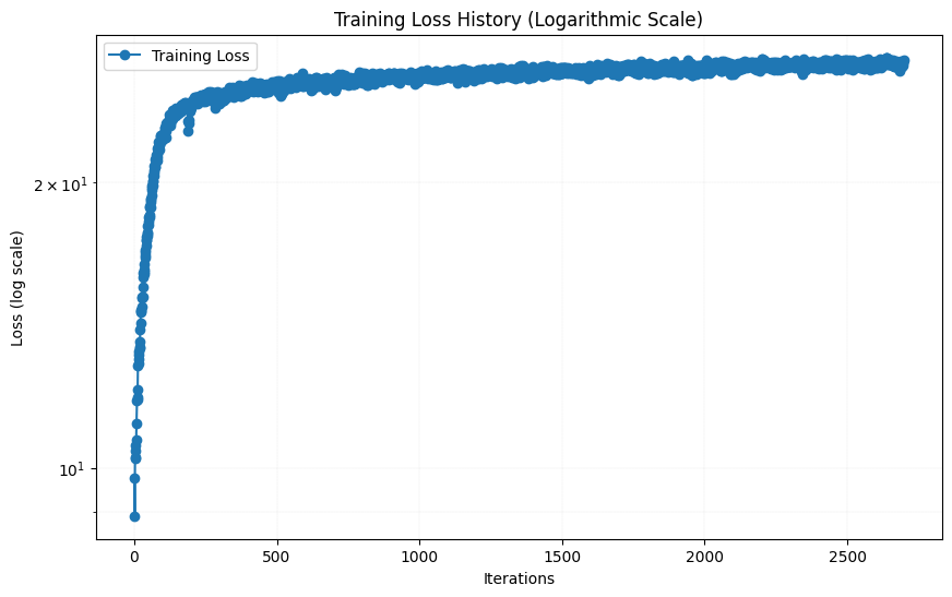
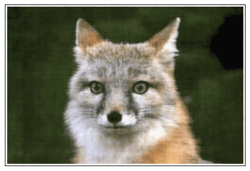
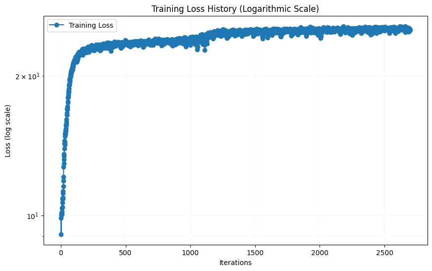
Both the number of hidden layers, the channel size, the L-value and the number of epochs are hyperparameters that can be tuned. I started with the initial values of 3 hidden layers, 256 hidden units, L = 10 and a learning rate of 1e-2. The result after 0, 10, 20, 30 and 38 epochs (around 3000 iterations) together with the evolution of the loss function (PSNR) are shown below: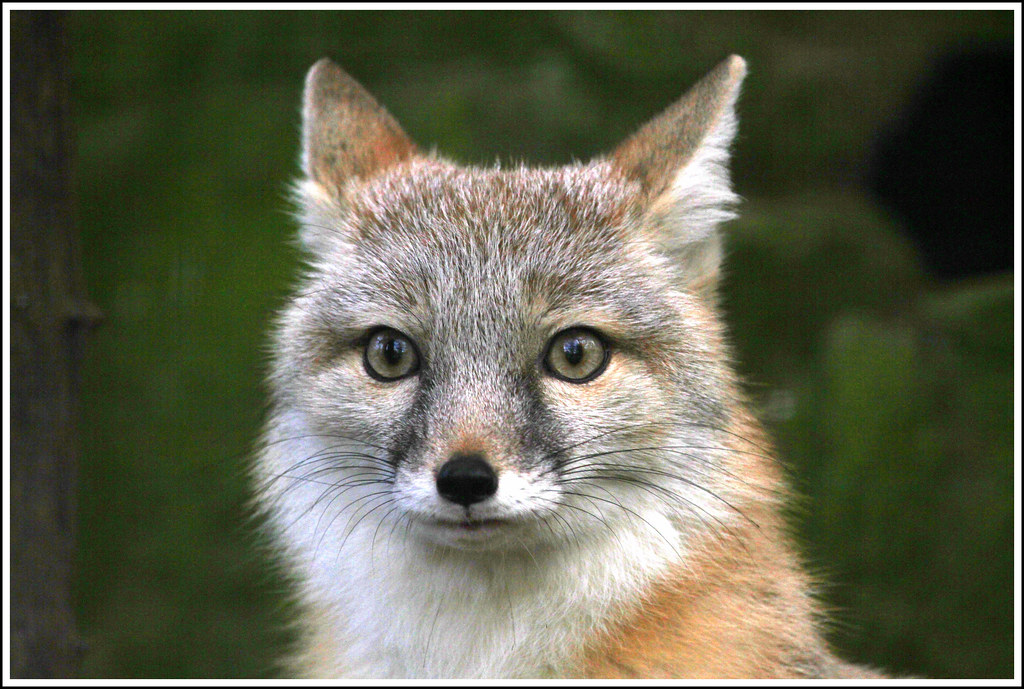


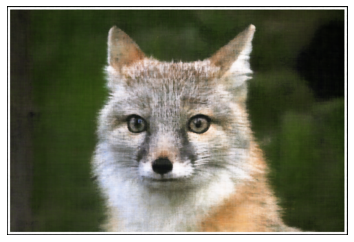
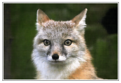
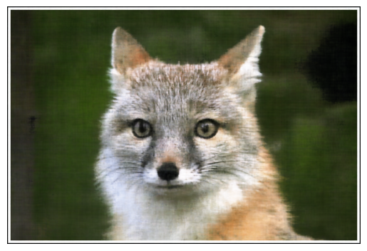
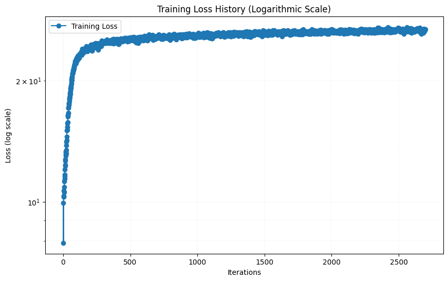
As we can see, the result after 38 epochs looks pretty good, although not completely as sharp as the original image. Then I tried changing some hyperparameters. I first tried changing the number of hidden layers from 4 to 6 by adding two more linear layers with 256 channels. The result after 38 epochs are shown below, together with the loss function are shown below:
The results were wors than the original model. The results were worse than the original model. This could be because adding two more layers increased the number of parameters, which likely requires more iterations to train the model effectively. I then tried increase L to 15, which increased the models input parameters from 42 to 62. The result after 38 epochs are shown below, together with the loss function are shown below:
The results looks almost indistingusihable from the initial hyperparameters, arguably slightly worse. The loss function looks to have flatten out ca as much as with the initial hyperparameters, so increasing the amount of iterations will likely not help much.
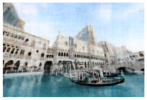
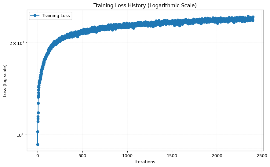
I then tried with another image of my choice. I decided a picture of the canal outside of the hotel "The Venetian" in Las Vegas. The result after 0, 10, 20, 30 and 38 epochs, as well as the resulting loss function, are shown below: I first tried to keep the initial hyperparameters for this image, i.e. 3 linear layers with 256 channels, L = 10 and a learning rate of 1e-2.

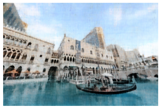


As the loss function did not fully flatten out after 38 epochs, I tried to increase the learning rate slightly to 1.2e-2. The result after 38 epochs are shown below:
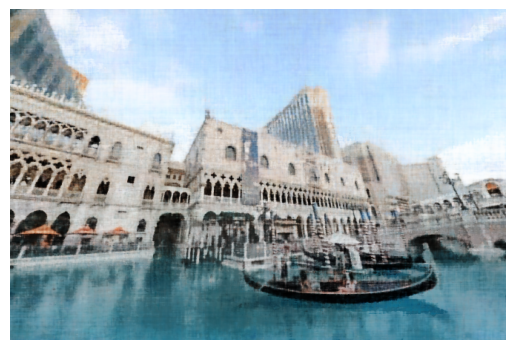
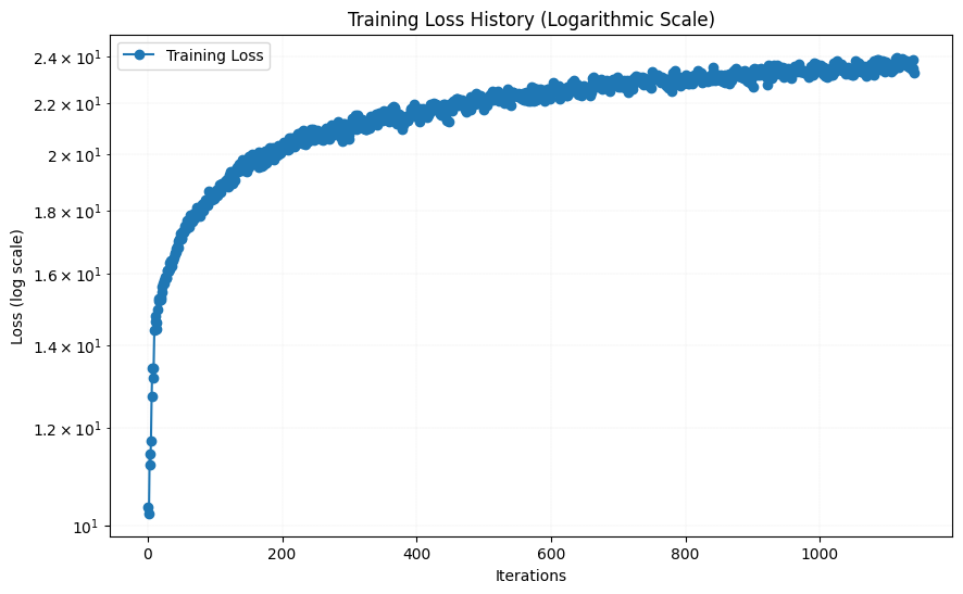
This result is very similar to a learning rate of 1.2. However, since the image size is smaller for the picture of The Venetian than for the picture of the fox, an equal amount of epochs leads to far less iterations. I therefore tried to increase the number of epochs to 80, while keeping the same initial hyperparameters. The result after 80 epochs, together with the loss function are shown below:
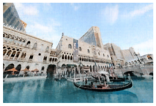
As for the fox, the recreation of the image of The Venetian were quite good, although this image is also a little blurry compared to the original.
Part 2: Fit a Neural Radiance Field from Multi-view Images
In this part of the assignment, we are going to create a 3-d video of a lego excavator based on 2-d images using a neural radiance field. A Neural Radiance Field (NeRF) is a deep learning model that generates 3D scenes by learning how light interacts with objects in space. It takes 3D coordinates and a viewing direction as input and predicts the color and density at those points. By sampling multiple points along camera rays and applying a physics-based volume rendering equation, NeRF synthesizes realistic 2D images from new viewpoints. These 2D immages can be used to create a 3D video. To set up this model, we first need to implement some functions:
Part 2.1 Create Rays from Cameras
First, we need a way to transfer from camera to world coordinates. This is done by multiplying with the camera to world matrix. The camera-to-world matrix is a 4x4 transformation matrix that includes the camera's rotation (3x3), translation (3x1), and a homogeneous coordinate row [0, 0, 0, 1], mapping 3D points from the camera's local coordinate system to the global world coordinate system.
The next function we need is a function that converts a point from the pixel coordinate system to the camera coordinate system. This is done by using the inverse of the camera matrix. The camera matrix is a 3x3 matrix that includes the camera's focal length, and the half-width and half-height of the camera. The inverse of the camera matrix is used to convert from pixel coordinates to camera coordinates. This is done by solving for u,v in the following equation: where K is given by: where fx, fy is the focal length and ox, oy is the half-width and half-height of the camera.
We also need a function that converts a pixel coordinate to a ray with origin and normalized direction. The origin is simply the position of the camera and can be found by using the above functions. The normalized direction is found by solving the following equation: where Xw is the pixel coordinate in world coordinates and ro is the camera position.
Part 2.2 Sampling and part 2.3, Putting the Dataloading All Together
Now that we are able to create rays from pixels from images, we need to sample points along the rays. We do this by 64 points uniformaly distributed along the ray, starting 2 units away from the camera and ending 6 units away from the camera. To avoid overfitting, we add a small, random pertubation to the points, but only during training. In order to sample random rays from the set of images, I made a class called RaysData that takes in images, K-matrices (intrinsic camera matrices), and camera-to-world matrices (extrinsic camera matrix). The class has a function sample_rays that samples N rays from random images and random pixels in the images.
Part 2.4: Neural Radiance Field
Now that we have 3d-samples, we want to use a nerual network (MLP also this time) to predict the density and color for those samples. This time, the MLP takes in 2 3-d vectors as input, the 3-d point and the viewing direction, and outputs the density and color. Both of the input vectors are applied Sinusoidal Positional Encoding (PE) to expand the dimensionality. For the position vector we use L = 10, and for the viewing direction we use L = 4. The MLP has 8 hidden layers with 256 hidden units and ReLU activation functions, before we split the model into two heads, one for density and one for color. The density head has one linear layer with 1 output unit, and the color head two hidden layers followed by a sigmoid. Since the direction is only used in the color head, we concatenate the position and direction vectors after the model is split. We also inject the position vector (after PE) in the middle of the MLP through concatination, to help the now deep neural network not forget about the input.
Part 2.5: Volume Rendering
The actual color of a pixel is calculated by integrating the color and density along the ray. This is done by using the volume rendering equation: This rendered color is what we want to compare with the actual color of the pixel. We do this by using the mean squared error loss function.
Results:
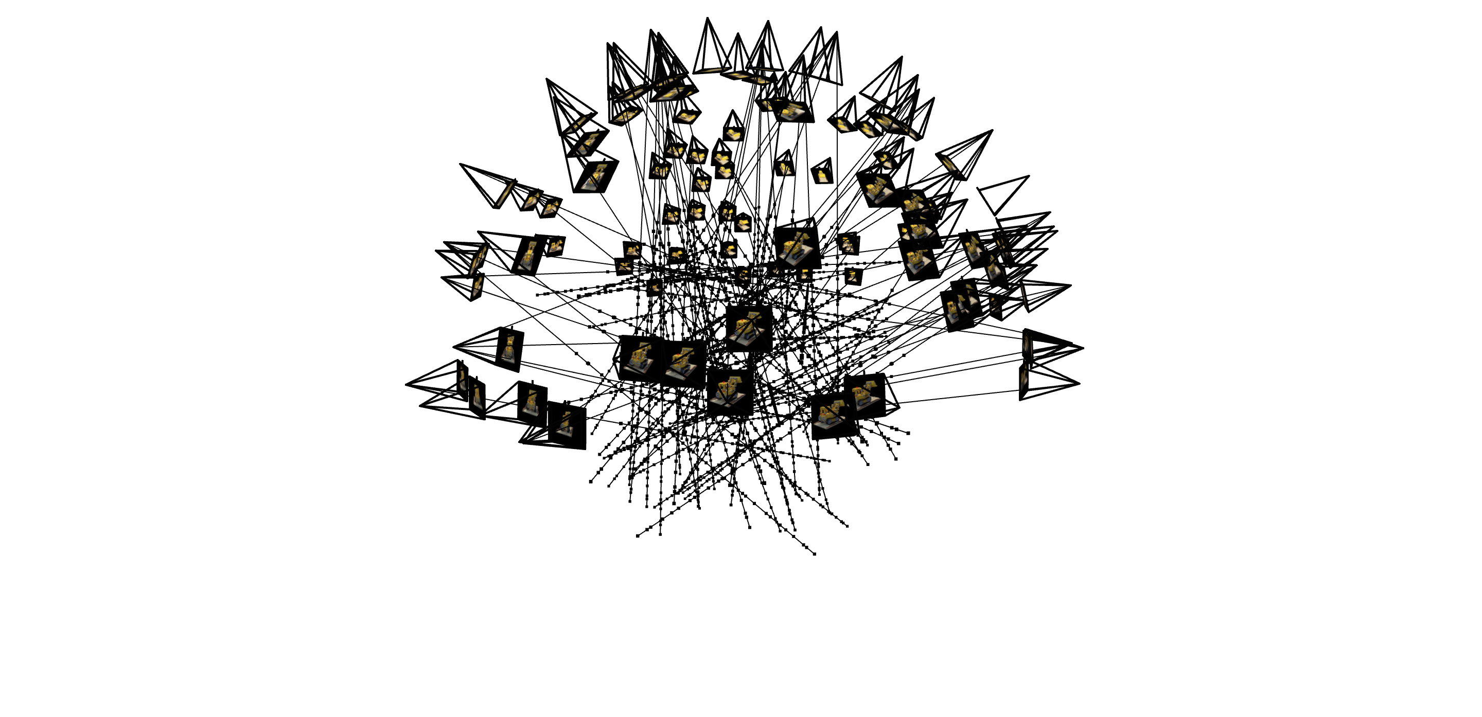
Below is a visulization of the rays and samples drawn at a single training step. In the actual training step, I used a batch size of 10000, but to make the visualization less drowded, I only show 100 rays and samples.
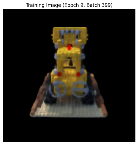
Here is the result from the training process on one of the training images every 50 iteration up to 350 iterations, and then every 400 iterations up to 4000 iterations. The model are trained on 10 epochs, resulting in 4000 iterations, with a learning rate of 1e-3, batch size of 10 000, 64 samples along each ray, and the rest of the hyperparameters as suggested in the project description. (L_x = 10, L_rd = 4 and the MLP just like the MLP in the picture of the project description). The PSNR on the training and validation data is also shown.
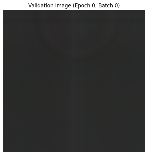
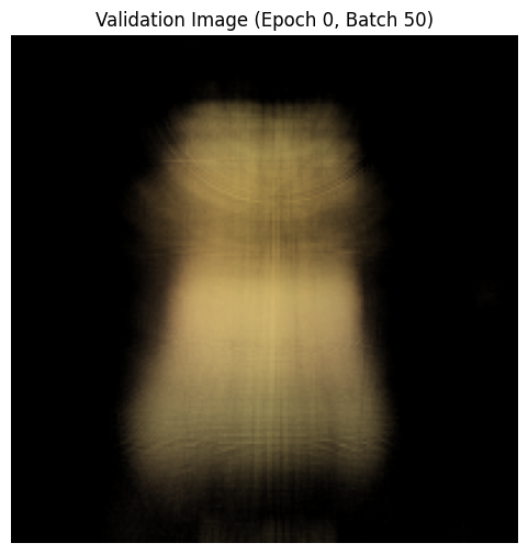
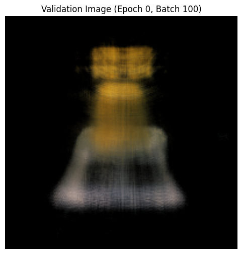
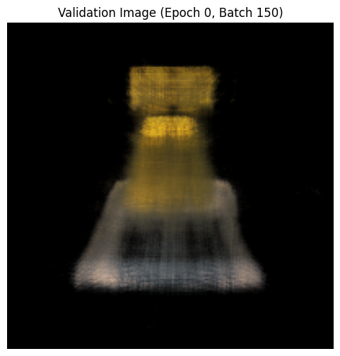
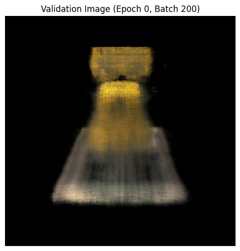
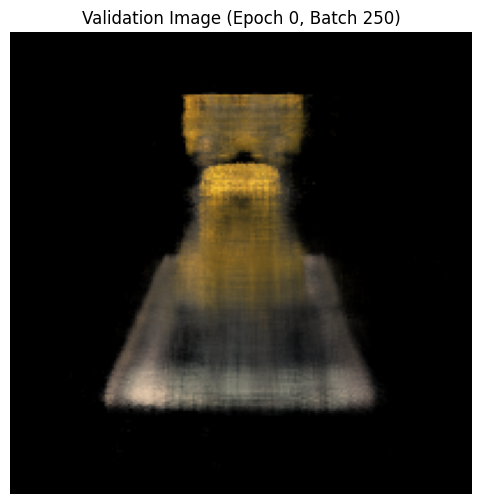
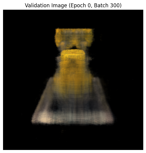
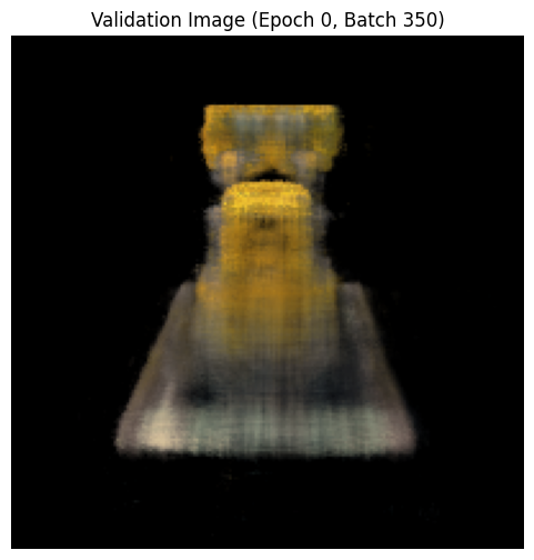


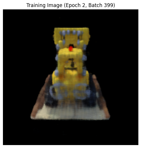
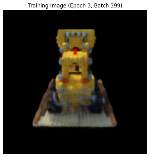
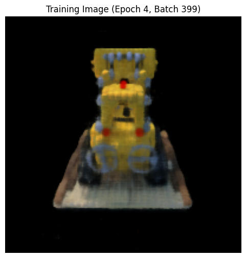

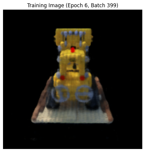

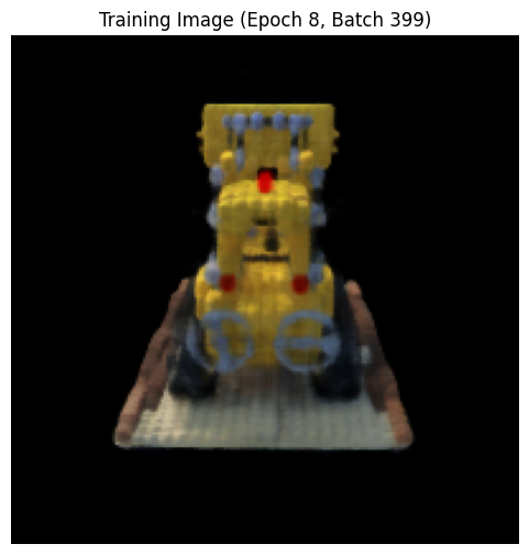
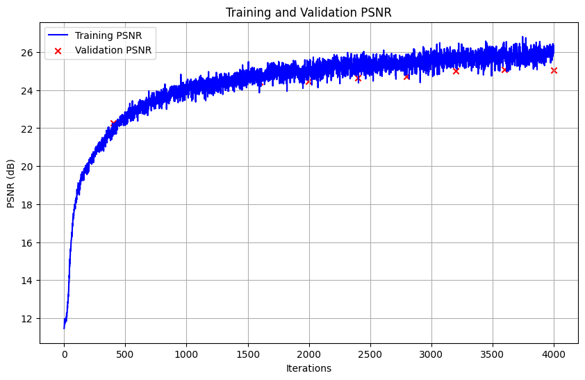
As expected, the images generated look more and more like the actual image the later in the training process we are. It is interesting to look at the plot of the PSNR on the training and validation data. In the first 1500 iterations, the PSNR is approximately the same for both the training and validaiton data. When we reach 2000 iterations, the PSNR for the validation data grows slower than for the training data, and after 3200 iterations the PSNR on the validation data stops increasing, and there appears to even be a slight decrese from 3600 to 4000 iterations. This suggests that the model is starting to overfit, which mean that there is no point of training the model further, unless we change the model architecture or the hyperparameters. The PSNR on the training data reached around 26 in the end, and the PSNR on the validation data reached around 25 in the end, which is both over the benchmark of 23, som I am happy with that!
Now finally, here is a spherical rendering of the lego using the test set. The videoes are generated after training the model for 4000 epochs (around 1 hour training). To see the videos, you need to open the html file in a browser, as the videos are not shown on the pdf.
I were pretty pleased with the result, as we can clearly see the lego excavator from all angles, including the details.
Bells & Whistles:
For Bells & Whistles, I decide to change the background color by rendering the Volrend function. This is done by picking the last sample for each cumulative transmittance along a ray. If the value on this is high, it means that a lot of light reamains unabsorbed, and we can therefore assume that the ray has not hit anything. Therefore we can simply add T_final*background color to the rendered colors, as this will not affect pixels that have hit an object (since T_final is close to 0). The resulting video with a different background color is shown below:
I am also quite pleased with the results from changing the background color, as the background is now clearly red, and the lego excavator is still as visible as before. However, we see some black stripes on the floor that are not present in the original images, so it is not perfect.